`bd.gwas.test`: Fast Ball Divergence Test for Multiple Hypothesis Tests
Yue Hu, Jin Zhu
2021/8/25
Source:vignettes/bd_gwas.Rmd
bd_gwas.RmdIntroduction
The
-sample
Ball Divergence (KBD) is a nonparametric method to test the differences
between
probability distributions. It is specially designed for metric-valued
and imbalanced data, which is consistent with the characteristics of the
GWAS data. It is computationally intensive for a large GWAS dataset
because of the ultra-high dimensionality of the data. Therefore, a fast
KBD Test for GWAS data implemented in function bd.gwas.test
is developed and programmed to accelerate the computational speed.
Faster implementation: quick start
We use a synthetic data to demonstrate the usage of
bd.gwas.test. In this example, phenotype data are generated
from three multivariate normal distributions with the same dimension but
heterogeneous mean and covariance matrix. The three multivariate normal
distributions are: (i).
,
(ii)
,
and (iii)
.
Here, the mean
is set to
and the covariance matrix covariance matrices follow the auto-regressive
structure with some perturbations:
The dimension of phenotype
is fixed as 100.
library(mvtnorm)

num <- 100
snp_num <- 200
k <- 100
rho <- 0.5
freq0 <- 0.75
d <- 3

set.seed(2021)

ar1 <- function (p, rho = 0.5)
{
    Sigma <- matrix(0, p, p)
    for (i in 1:p) {
        for (j in 1:p) {
            Sigma[i, j] <- rho^(abs(i - j))
        }
    }
    return(Sigma)
}

mean0 <- rep(0, k)
mean1 <- rep(0.1 * d, k)
mean2 <- rep(-0.1 * d, k)

cov0 <- ar1(p = k, rho = rho)
cov1 <- ar1(p = k, rho = rho - 0.1 * d)
cov2 <- ar1(p = k, rho = rho + 0.1 * d)

p1 <- freq0 ^ 2
p2 <- 2 * freq0 * (1 - freq0)
n1 <- round(num * p1)
n2 <- round(num * p2)
n3 <- num - n1 - n2
x0 <- rmvnorm(n1, mean = mean0, sigma = cov0)
x1 <- rmvnorm(n2, mean = mean1, sigma = cov1)
x2 <- rmvnorm(n3, mean = mean2, sigma = cov2)
x <- rbind(x0, x1, x2)
head(x[, 1:6])
## [,1] [,2] [,3] [,4] [,5] [,6]
## [1,] 0.07039579 0.6100092 0.5546911 0.5346480 0.5785020 -1.3470882
## [2,] -0.19620313 0.2196482 -0.2968494 -0.7916355 -1.3371275 -0.5766259
## [3,] -0.18575434 -1.4601779 -1.2635876 -0.8933793 -0.9336481 -0.5277624
## [4,] 1.56843201 1.6330457 1.8725853 0.8344465 0.5674250 -0.3928510
## [5,] -0.54939765 0.1602176 0.4325440 -0.1750343 0.5231533 -1.0931093
## [6,] -0.19665796 -1.3788672 -0.6887342 -1.2731113 -0.6638883 0.0764279The number of SNPs is fixed as and the sample size is set to . The sample sizes of the three groups follow the transmission ratio: Here, is set to be , representing a scenario that close to the real data. is a user-specific positive integer, indicating the differences between the three probability distributions. Here, we use , aiming to show that the SNP which matched with the distribution can be identified, even when the differences between distribution is small.
effect_snp <- c(rep(0, n1), rep(1, n2),
                rep(2, n3))
noise_snp <- sapply(2:snp_num, function(j) {
  sample(
    0:2,
    size = num,
    replace = TRUE,
    prob = c(p1, p2, 1 - p1 - p2)
  )
})
snp <- cbind(effect_snp, noise_snp)
head(snp[, 1:6])
## effect_snp
## [1,] 0 1 0 0 0 0
## [2,] 0 1 1 1 0 0
## [3,] 0 0 0 1 0 0
## [4,] 0 0 1 0 2 0
## [5,] 0 1 1 0 0 0
## [6,] 0 1 1 1 1 0Given the synthetic dataset x and snp,
multiple KBD tests is conducted by:
library(Ball)
res <- bd.gwas.test(x = x, snp = snp)
## =========== Pre-screening SNPs ===========
## Refining SNP... Progress: 1/1.
## Refined p-value: 0.0000499975, cost time: 2 (s).And we present the SNPs that is significant:
str(res)## List of 8
## $ statistic : num [1:200] 4.218 0.876 1.881 1.104 1.143 ...
## $ permuted.statistic :'data.frame': 20000 obs. of 1 variable:
## ..$ g3: num [1:20000] 0.819 1.114 1.112 1.563 0.906 ...
## $ eigenvalue : NULL
## $ p.value : num [1:200] 0.00005 0.9112 0.0577 0.60847 0.55267 ...
## $ refined.snp : int 1
## $ refined.p.value : num 5e-05
## $ refined.permuted.statistic: num [1:20000, 1] 1.216 0.857 0.988 0.937 1.37 ...
## ..- attr(*, "dimnames")=List of 2
## .. ..$ : NULL
## .. ..$ : chr "SNP1"
## $ screening.result :List of 5
## ..$ : num [1:200] 4.218 0.876 1.881 1.104 1.143 ...
## ..$ :'data.frame': 20000 obs. of 1 variable:
## .. ..$ g3: num [1:20000] 0.819 1.114 1.112 1.563 0.906 ...
## ..$ : num [1:200] 0.00005 0.9112 0.0577 0.60847 0.55267 ...
## ..$ : int [1:10000] 0 97 44 35 95 99 39 19 46 65 ...
## ..$ : int 0Why bd.gwas.test is faster?
Our faster implementation for multiple testing significantly speeds up the KBD test in two aspects.
Two-step algorithm
First, it uses a two-step algorithm for KBD. The algorithm first computes an empirical -value for each SNP using a modest number of permutations which gives precise enough estimates of the -values above a threshold. Then, the SNPs with first stage -values being less than the threshold are moved to the second stage for a far greater number of permutations.
Recycle permutation result
Another key technique in bd.test.gwas is reusing the
empirical KBD’s distribution under the null hypothesis. This technique
is particularly helpful for decreasing computational burden when the
number of factors
is very large and
is a single digit. A typical case is the GWAS study, in which
or
but
.
Power evaluation
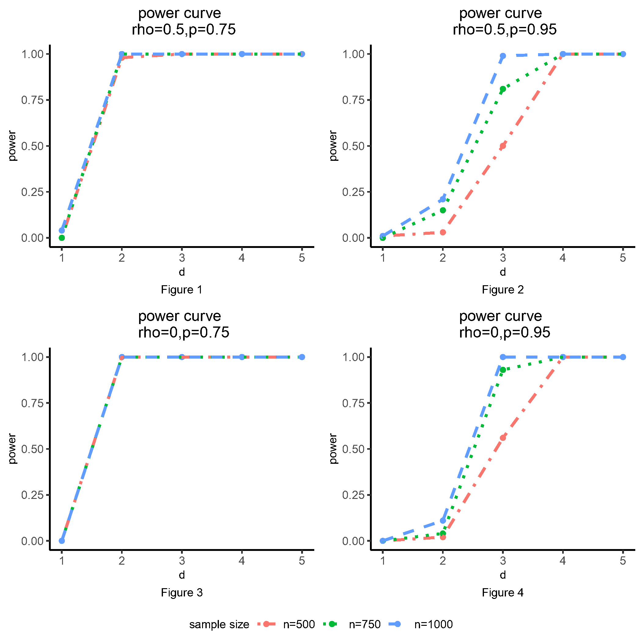
According to the simulations:
the empirical type I errors of KBD are reasonably controlled around ;
the power of KBD increases as either the sample size or the difference between means or covariance matrices increases. The empirical power is close to when the difference between distributions is large enough.
Furthermore, correlated responses may slightly decrease the power of the test compared to the case of independent responses. Moreover, KBD performs better when the data are not extremely imbalanced and it maintains reasonable power for the imbalanced setting.
Compared to other methods, KBD performs better in most of the scenarios, especially when the simulation setting is close to the real data. Moreover, KBD is more computationally efficient in identifying significant variants.
From Figures 1 and 3, we can notice that the power curves are similar after sample size of 500, when the minor allele frequency is not small. On the other hand, when the minor allele is rare, a larger sample size can lead to a higher power from Figures 2 and 4. The four figures show how sample size could affect the power of the KBD method, indicating that there is an inverse relationship between minor allele frequency and the sample sizes in order to get sufficient power.
Conclusion
We implement bd.test.gwas in Ball package for handling
multiple KBD test. KBD is a powerful method that can detect the
significant variants with a controllable type I error regardless if the
data are balanced or not.
Reference
Yue Hu, Haizhu Tan, Cai Li, Heping Zhang. (2021). Identifying genetic risk variants associated with brain volumetric phenotypes via K-sample Ball Divergence method. Genetic Epidemiology, 1–11. https://doi.org/10.1002/gepi.22423